All-wheel drive coupling Haldex generation V

When driving in difficult conditions such as snow, ice and mud, a conventional two-wheel drive vehicle will not cope. For increased safety and performance, many car manufacturers offer an all-wheel drive alternative. However, there is a wide variety of four-wheel drive setups. Some systems are all-wheel drive, which means that all wheels receive torque from the engine at all times. The amount of torque distributed between the front and rear axles can have a fixed ratio, usually 50/50, or be variable. Such full-time systems are common among Asian automakers such as Subaru and Toyota. As an alternative to full-time systems, there are systems called part-time. Vehicles using the part-time system can be either front- or rear-wheel drive under normal driving conditions. To distribute the torque to the other axle, some kind of torque transfer device is required. There are many different solutions to how this can be achieved. To transfer the torque between the right and left wheels, a differential is needed, capable of distributing the available torque.

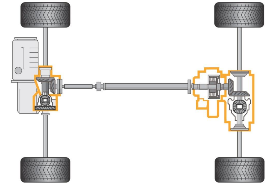
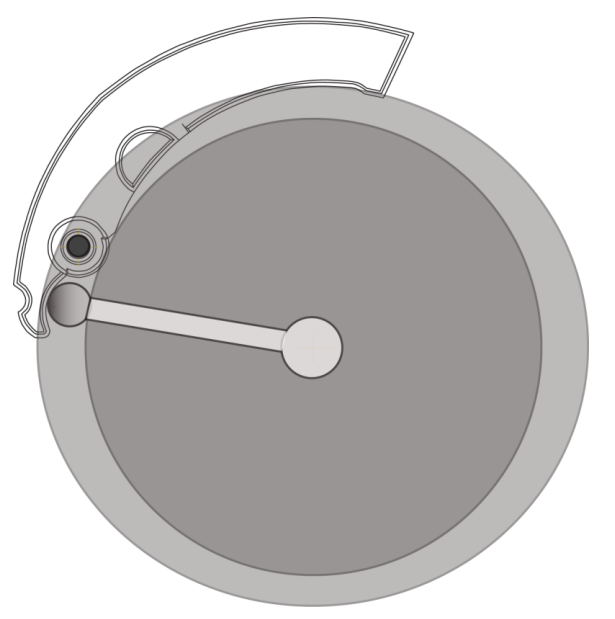
Illustration of a transmission. The highlighted areas are the rear and front differentials and the all-wheel drive clutch:

In modern cars, these systems are usually integrated with other systems such as ABS and ESP. These systems receive data from a number of on-board sensors. If the car begins to skid, the system automatically turns on and helps the driver to stabilize the car.

In addition to increased safety, one of the benefits of the part-time system is slightly reduced fuel consumption due to reduced transmission losses. On the other hand, the part-time system is more difficult to control and often suffers from delays. It needs a fast and reliable control strategy to prevent unexpected system behavior.

During the disassembly of such algorithms, the system model is of great importance. Time and money can be saved by reducing the need to test software directly on the system.

History of the company

The Haldex concern was created in 1985 by the merger of three Swedish companies: Garphyttan, Haldex and Hesselman. At the time, the main source of profit was the spring wire industry, which accounted for 50 percent of total sales. However, the division was sold in 2009, and now the main revenue comes from the Traction and Hydraulics divisions. After the acquisition of Barnes Corp in 1987 and Vickers in 1991, the hydraulic part of the concern was created. The patent for the new four-wheel drive was purchased in 1992. The first generation clutch was released to the market in 1998. In the same year, Haldex Traction Systems was established as a division of the Haldex concern.

Traction systems Haldex

The patent, acquired by Haldex in 1992, was bought from former rally driver Sigge Johansson. The basic idea was for the clutch to be actuated by a pump that was driven by the difference in wheel speeds. Haldex developed the clutch in close cooperation with Volkswagen. In 1998, serial production of the 1st generation clutch began. Since then, many companies have used clutches in their cars, including Volvo, Ford, Bugatti and SAAB/GM [2]. Since 1998, the clutch has been improved, and now the fifth generation is being developed. In 2009, Haldex announced a SEK 4.5 billion deal with Volkswagen to provide the next platform with this fifth-generation system.

Previous generations

The first two generations of four-wheel drive are quite similar and are driven by the difference in wheel speed. This motion drives a hydraulic pump that creates flow and actuates the LSC. This means that these systems are reactive, meaning wheel slip must occur before the system is activated. 1/4 turn of the wheel creates enough flow to lock the axle completely. The pressure level in the LSC is controlled by the ECU and regulated by a linear throttle. Generation II is a further development of the first generation, but with more sensors and an electromagnetic proportional valve, the overall performance has been increased. To reduce response times even further, Haldex has introduced a generation III with pre-tensioning capabilities, the PreX. The addition of a small feed pump, which allows torque to be delivered to the rear wheels even when the wheel is not slipping, has reduced response time. With the addition of this feature, the system is now proactive, meaning it is able to adjust the need for all-wheel drive in real time based on information provided by on-board sensors.

Generation IV

With the Haldex IV generation, a unique all-wheel drive system was introduced. The system is described as intelligent and able to sense the driver's intentions. The torque is distributed between the four wheels all the time. However, the distribution can be from 2% of the total to 85% on one rear wheel. By transferring only 4% of the torque to the rear axle while driving, energy consumption is reduced. And if sliding occurs on three tires at the same time, as much of the available torque as possible is transferred to the tire that has the grip. This distribution between the rear wheels is controlled by a multi-plate clutch that is regulated by hydraulic pressure. In previous generations of this, there were complaints about delayed response times. It was because we couldn't build up the pressure fast enough. By introducing an accumulator with a separate feed pump, high pressure can be instantly available for control use. This control is performed by the electrical control unit (ECU). Using more than 20 sensors around the car, the ECU updates the torque distribution 100 times per second.

Generation V

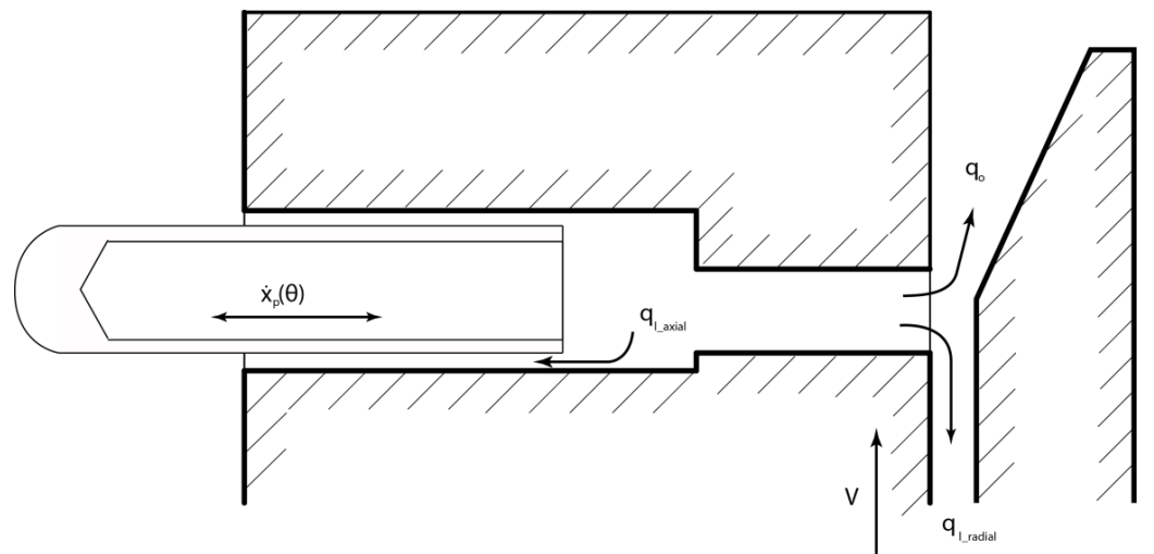
To reduce weight and space, the battery and control valve added to the fourth-generation clutch have now been removed. Instead, pressure must be created directly in the clutch pack by a specially designed feed pump. A pump is a machine that creates a flow, the medium that flows is hydraulic oil. Clutch pack pressure is created when oil is pumped into a chamber containing a piston that transmits this pressure to the discs. To maintain a sufficiently low response time, the pump has a design in which the fluid flow has two different paths through which it can be directed. When a stable pressure state is reached, the fluid no longer enters the clutch, but is only pumped out into the surrounding system. When pressure is required, the outlet closes and all flow enters the clutch pack.

Theory and modeling

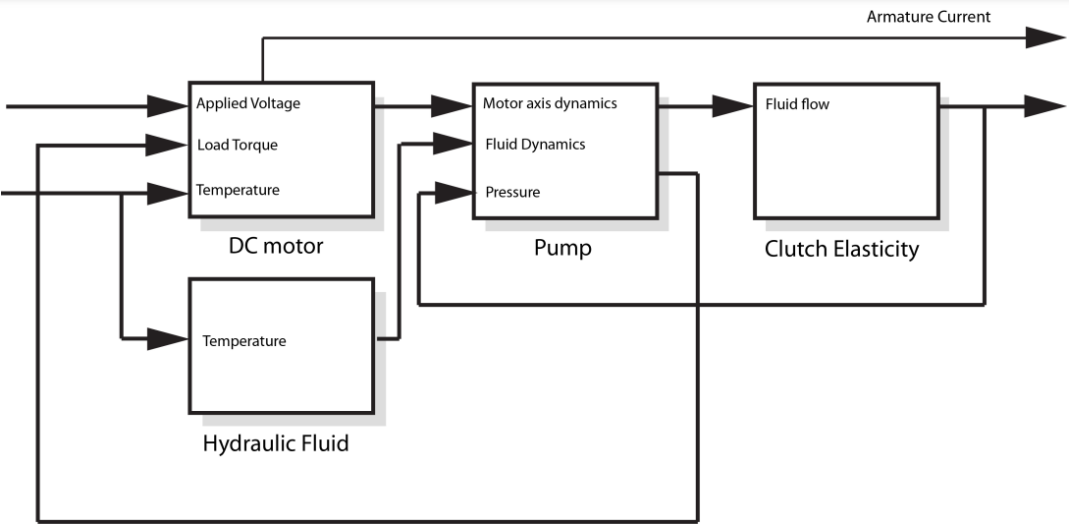
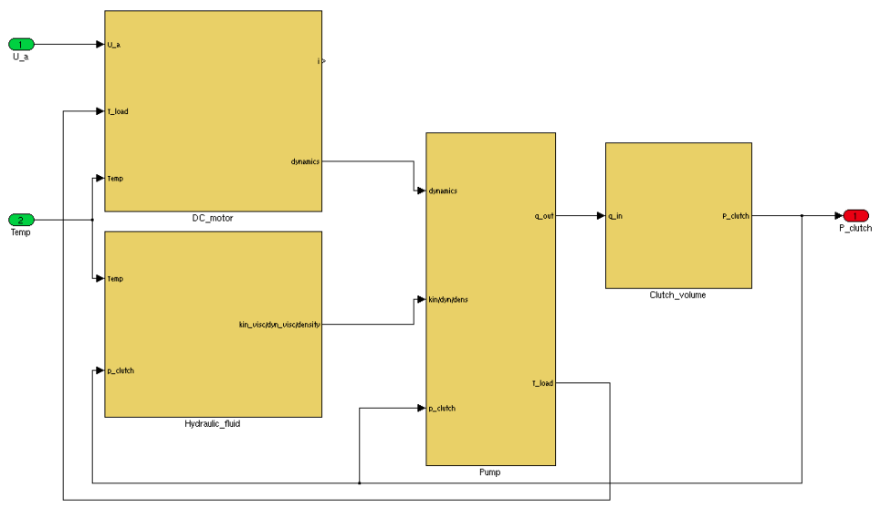
The complete model will consist of four subsystems: engine, pump, oil and multi-plate clutch. You can view a modified version of the original schematic that illustrates the Gen V system. The first system will be the electric motor. The signals coming to this subsystem are armature voltage and temperature. These signals are also signals in the full model. The outputs from the motor subsystem are armature current and motor axis dynamics, i.e. rotational speed, axis acceleration and position.

Scheme of clutch Gen. V Haldex:

The dynamics of the engine axis are entered into the pump subsystem together with the dynamics of the oil and clutch pressure. Pump output is the net flow entering or leaving the pump. This flow is the input of the coupling model, which has the coupling pressure as output. This pressure is then fed back to the pump. The subsystem that calculates the oil dynamics takes the temperature as an input and then connects to the pump. The output of the full model is the coupling pressure and the armature current.

Structural diagram of subsystems of complete models:

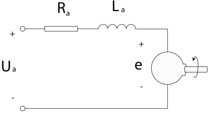
Direct current machine

A DC machine is often used as an actuator throughout industry today. The fundamental design of the machine makes it durable and less likely to malfunction or break during operation. It also has a near-linear armature voltage-to-speed relationship and a near-linear current-to-torque relationship, making it relatively easy to control. In this chapter, the generator pump drive will be considered. V all-wheel drive system. First, there will be a brief description of the working principle of the DC machine, followed by a review of the motor equations. Gene. The V motor is a 12-pole permanent magnet DC machine. Since actual operating time data is not available, the standard engine equations will be used to model the engine. Some additions will be made regarding the different types of friction. The model implemented in Simulink also takes into account different types of ambient temperature. Data for this was provided by the manufacturer.

Principle of operation

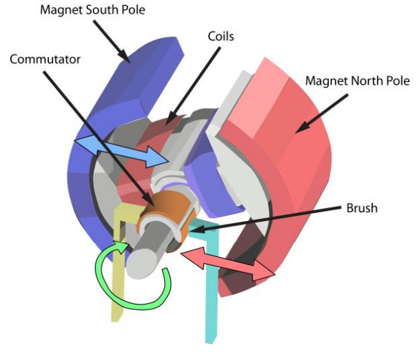
A PMDC motor consists of windings mounted on a rotor, several north and south pole magnets arranged in pairs, and a commutator. Permanent magnets are installed around the stator. The commutator is a set of copper conductors fixed to the rotor. Current is transferred to the commutator through a pair of carbon brushes that slide across the surface of the commutator as the rotor rotates. When the brushes change the plate, the current in the coils changes direction. Since the current in the coil creates a magnetic field, changing the direction of the current also changes the polarity of that magnetic field. Arranging the coils and commutators so that the induced magnetic field attracts or repels the magnets in the stator creates a torque.

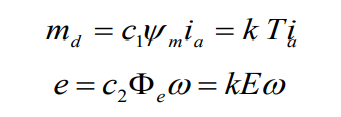
Governing equations

The differential equations describe the armature current, ia, the induced armature voltage, ua, and the electric torque, md.

Equation:

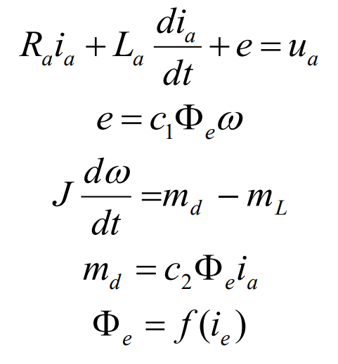
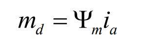
where mL is the load moment on the motor axis. This model is one of the DC machines with a separate output and therefore also includes a function for electric magnetic flux. Since the engine in the Gen V is a PMDC engine.

Equation:

We get the final current equation:

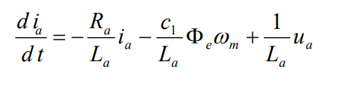
The DC motor manufacturer provided temperature dependent data and constants for the motor. The corresponding constants are the torque constant kT and the voltage constant kE.

Friction and losses

The equations presented in the previous section do not include any motor losses. There are two types of friction losses [4]; viscous damping and dynamic moment of friction. Both of them depend on the temperature. Viscous damping is the frictional moment caused by the lubricating fluid and the moving parts of the engine and is assumed to be directly proportional to speed. The dynamic moment of friction is the Coulomb friction and is considered a constant term that adds to the losses.

Adding these conditions and introducing new notations, we get the final torque equation:

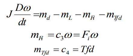
Where mFi is the viscous damping and mTfd is the moment of dynamic friction.

Other phenomena such as eddy currents and field weakening will also cause losses. Eddy currents occur when a conductor undergoes a change in magnetic flux. This can cause current to circulate inside the conductor. These circulating currents create a magnetic field that opposes the magnetic flux from the permanent magnet. Field weakening occurs when current flows through the coil windings. The current creates a magnetic field that distorts and weakens the field in the same way that eddy currents do. Due to the lack of experimental data, the influence of these phenomena will be neglected.

Final motor equations

With the use of equations and new notations, the basic equations for a DC machine are obtained:

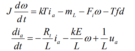
where Rt, kE and kT are temperature-dependent parameters.

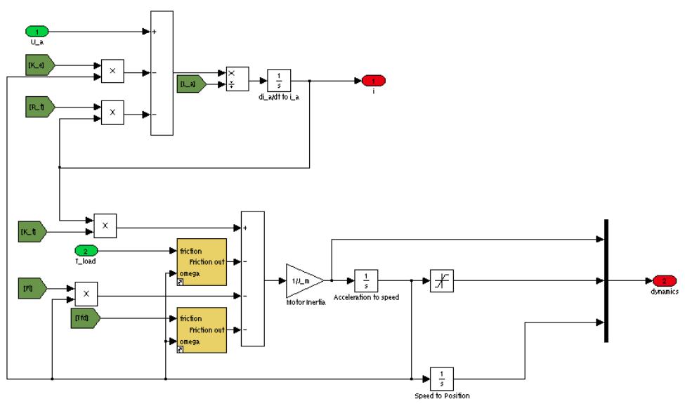
Simulink model

The motor block in the Simulink model has three inputs: armature voltage u_a, pump load T_load, and motor temperature Temp. The last input affects the previously mentioned temperature-dependent parameters. Inside the block, a lookup table is used for each of these parameters, using Temp as input. The output signals of the unit are the armature current, the effective load torque produced by the machine, and the rotational speed and angular position of the shaft.

Hydraulic pump

An axial-piston pump consists of three main components: a housing containing pistons, a pump cover and a tipping plate [6]. The angle of the diverter plate determines the working volume of the pump and can be variable or fixed. On the Gen V pump, the swashplate is a fixed-angle angular thrust bearing. The barrel is held near the pump cover, which contains the suction and discharge holes. The arrangement of these ports is such that the suction port is connected to the low pressure side of the system and the discharge port is connected to the high pressure side. When the barrel rotates, the pistons slide along the swash plate. The angle of the swash plate forces the pistons to make reciprocating movements back and forth, which creates a pumping action, that is, the suction of liquid from the low pressure side, its release from the high pressure side.

Cross-section of the transfer plate, barrel, pistons and pump cover:

As mentioned in the introduction, a pump is a machine that creates flow. This flow creates pressure in the clutch chamber. Once the desired pressure is reached in the coupling, the flow created by the pump needs an alternative path, otherwise it will continue to build pressure. The center of the Gen V pump barrel is hollow, and fluid under pressure can reach this chamber. From this chamber, three drilled channels lead the liquid to the surface of the barrel. There are three arms-lever on the surface that rotate together with the barrel. They are designed to control the opening and closing of channel openings. If the rotation speed is high enough, the centripetal force turns the lever and pushes the ball located on its shorter end into the outlet, thereby closing it. As the pressure in the chamber increases, the force of the fluid causes a rotational motion in the opposite direction to the centrifugal force. This opens the outlet and allows it to flow into the surrounding system. The shoulders also act as check valves, when pumping stops, the high pressure created in the system will lift the shoulders, thus creating a high flow through the channel openings and causing a rapid pressure drop.

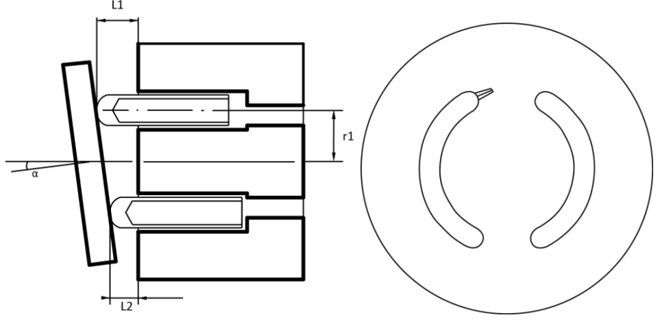
Piston position

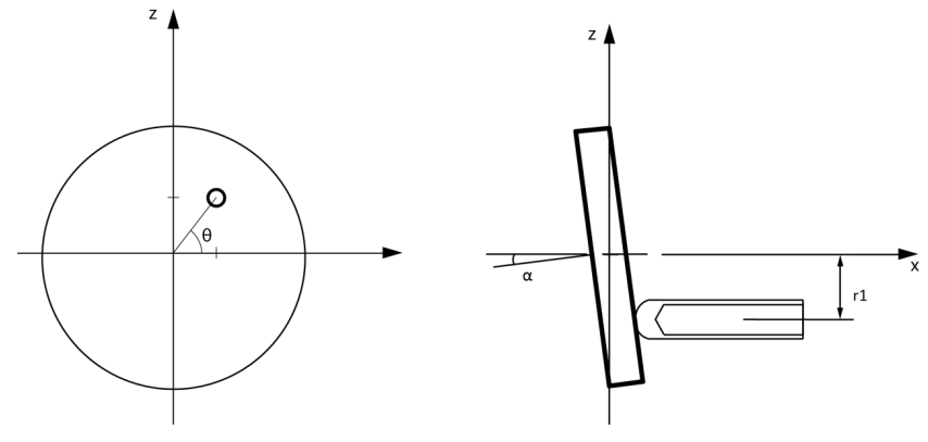
To accurately account for the forces acting on the piston, it is necessary to establish a coordinate system for the pump cylinder, swashplate and piston position. The defined x, y, z plane has the x axis in the direction of the DC machine shaft. Coordinate system.

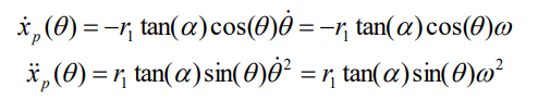
By studying the diagram, you can determine the axial position of the piston:

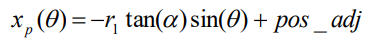
where r1 is the radius from the center of the barrel to the pistons, and α is the angle of inclination of the washer. This gives a position that oscillates between a positive and negative value. The pos_adj constant is then added to balance the position which is zero at BDC. Since velocity and acceleration will be needed to calculate the forces acting on the piston, this works out.

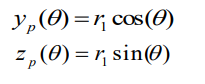
The y and z coordinates are simple:

Piston forces

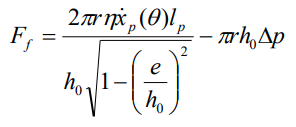
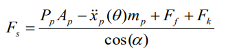
Having drawn up the equilibrium equation of the system, it is possible to determine the forces acting on it. The equilibrium equation in the x direction is established.

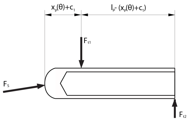
The frictional force due to viscosity in the cylinder when the piston moves inside is given by the following equation. The main parameters governing this equation are the viscosity η, the average piston-to-cylinder clearance h0, and the piston speed px.

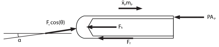
The force in the z direction can be calculated as a function of the axial angle. It is assumed that the reaction forces of the barrel on the piston are located in the innermost part of the piston and at the point where the piston exits the barrel. Having drawn up the equilibrium equation of the piston, the moment equation can be established.

Forces acting on the piston in the z direction:

It turns out:

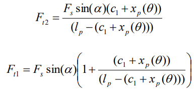
These forces Ft1 and Ft2 will be used to calculate the friction losses in the piston chamber.

The spring force equation:

After rearranging the equation, we get the expression for the force acting on the tipping plate:

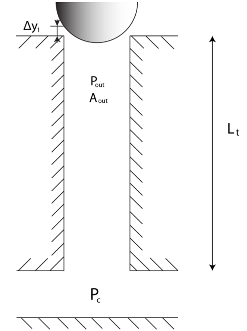
Lever

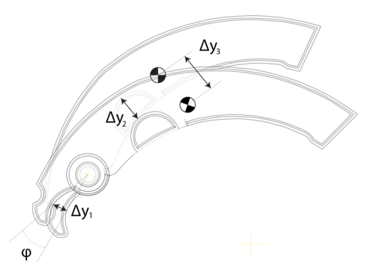
The purpose of this section is to calculate the flow exiting through the hole in the sleeves. This flow is regulated by the area of the opening at the end of the channel. This area, in turn, is regulated by Δy1, which is the height between the hole and the ball at the end of the lever arm. The balance equation for the arm is illustrated using the pin hole as the center of rotation:

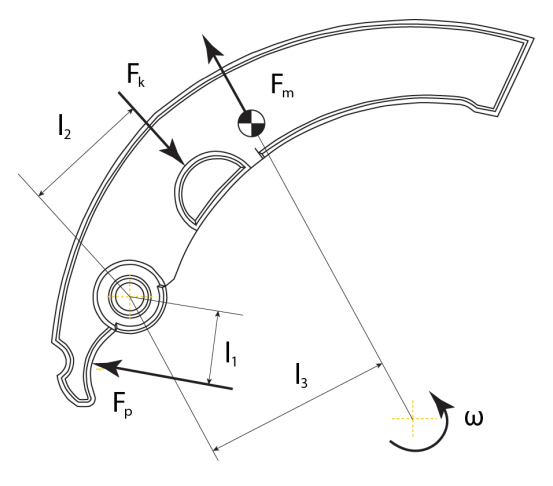
These forces are given by:

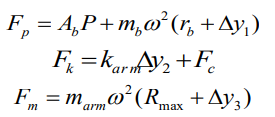
where Ab depends on the height between the outlet and the bullet. To make all equations dependent on this height, we form the following simplifications and relations:

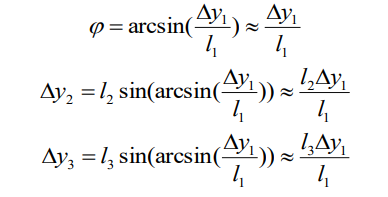
The simplification of the equations is due to the small angle changes that will occur during operation:

Hagen-Poiseil

Hagen-Poiseuille describes the laminar flow of an incompressible fluid in a pipe. Using this flow equation, the pressure drop in the channel leading to the orifice can be calculated. Assuming a known flow Q and channel geometry, the Hagen-Poiseuille flow with our notation becomes:

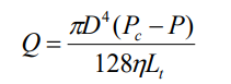
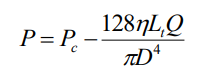
where η is viscosity, D is pipe diameter, Lt is pipe length, Pc and P are different pressures . This can be changed to:

Cross-section of the pressure channel in the pump barrel:

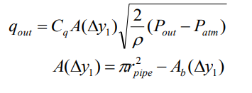
Flow equation

Ultimately, this leads to the flow equation. The flow through the orifice is defined as:

Engine load moment

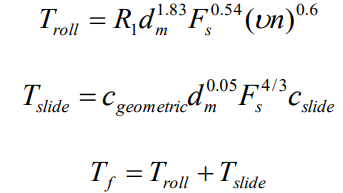
The total load torque acting on the motor shaft consists of four different torques: the viscous torque Tv caused by the fluid movement in the pump, the friction torque in the bearings and other parts moving against each other Tf, and the torque , caused by inertia. YOU All this depends on the speed of rotation or acceleration of the shaft.

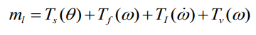
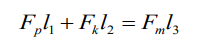
The equilibrium equation for the torque around the motor shaft is illustrated. The contribution of piston forces to the total torque Ts is described by:

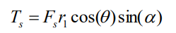
where α is the angle of inclination of the plate, and the length of the shoulder is described by r1cos(θ) .

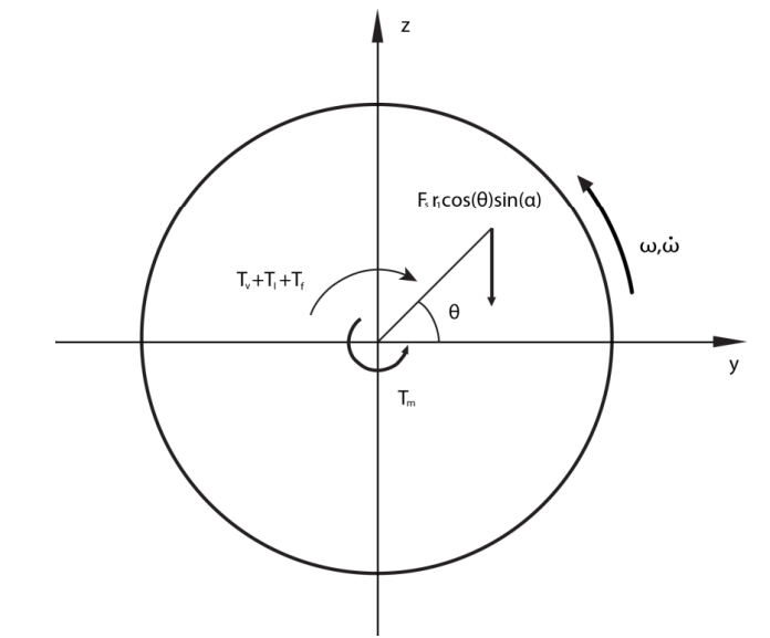
The friction moment in the thrust thrust bearing is calculated according to the empirical relations provided by SKF and is determined by the formula:

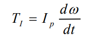
The torque due to viscosity Tf, since no empirical relations can be found for it, is estimated as a function of rotational speed and acceleration. The inertia Ip of the bearings, barrel and pistons was calculated using the CAD system and set to a constant value. The equation for this contribution is defined as:

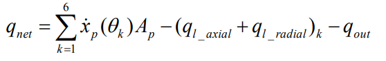
Piston flow and leaks

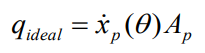
As the barrel begins to rotate, the pistons are forced to reciprocate back and forth, creating a pumping action. The ideal flow that can be provided by one piston is described by the equation:

The leak flows in the pump:

All hydraulic pumps have internal leaks. To account for these internal losses, leakage in the axial direction between the piston and cylinder is introduced, as well as leakage in the radial direction.

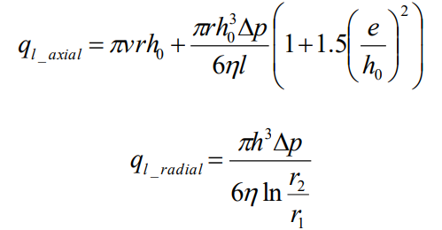
The eccentricity e of the piston is assumed to be zero, so the equation can be simplified as follows:

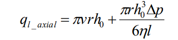
The net pump flow can now be described by the equation:

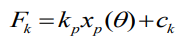
Clutch package and system pressure

There is an elasticity of the pressure created in the coupling. Different clutch packs have different elasticity depending on drivetrain, clutch housing, wear and number of discs used. Therefore, the dynamics of the clutch package must be included in the model.

Haldex conducted a series of tests to establish the elasticity ratio by pressurizing the clutch pack and measuring the volumetric expansion. These measurements contain a general characteristic, including oil elasticity. The elasticity data used in this simulation is based on the characteristics of the clutch package developed for Volkswagen. A certain volume of hydraulic fluid in the clutch pack corresponds to the pressure level, that is, the pressure in the system is a function of the volume. The flux is integrated over time, thus representing the volume, and used as input to a lookup table containing the elasticity data. The output signal is the pressure in the system, which is then fed back to the model.

Simulink model

The Simulink pump model is divided into three subsystems. First, the piston position, acceleration and velocity are calculated. They are sent to the unit that calculates the load on the motor shaft and also to the unit that calculates the flow from the pump.

Hydraulic fluid

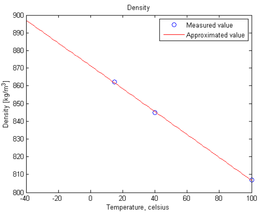
Since the model must work in a wide range of temperatures, the properties of the hydraulic fluid become essential. The properties modeled are density, viscosity, and bulk modulus. Since density measurements were available, the density is modeled as a function of temperature, even though the hydraulic fluid can be assumed to be incompressible with very small density variations as a consequence. Viscosity has a significant temperature dependence and is approximated based on Haldex measurements.

Governing equations

The properties of liquids are very complex, and physics is considered to be beyond the scope of this master's thesis. Thus, the mathematical model is based on empirical relationships and experimental data.

Density

Density is used to calculate dynamic viscosity. It is approximated by a linear function of temperature.

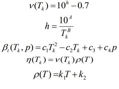
Viscosity

Viscosity is a measure of internal friction in a fluid and affects the performance of a hydraulic pump. Kinematic viscosity, ν, is calculated according to the ratio:

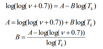
Knowing the kinematic viscosity at two different temperatures, Tk, the constants A and B can be determined.

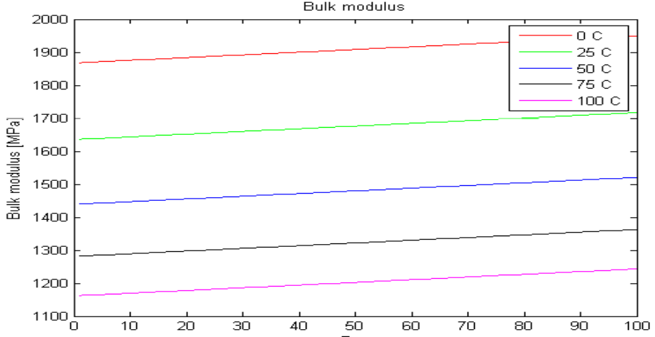
Volumetric module

The bulk modulus is a measure of fluid compressibility and depends on both pressure and temperature. Since no experimental data were available, the bulk modulus was modeled according to data found by Olsson O. and Rydberg KE and approximated by a quadratic function of temperature and pressure.

Decision

Solving equation 3.58 gives the final equation for viscosity, bulk modulus, and density. The constants c1-c4, k1 and k2, are used to approximate the function:

Completed model

General model

The complete model, like the actual equipment, is controlled by the rotation of the motor shaft. By using the engine equations to solve for the shaft angle, velocity, and acceleration, the axial position, velocity, and acceleration of each individual piston can be determined. These are then used to calculate the load torque and flow produced by each piston. Adding these flows generates the total flow. Total flow into or out of the clutch is calculated by subtracting the flow coming out of the lever arm hole. This flow is used to estimate the amount of fluid inside the coupling, which in turn is used to calculate the pressure acting on the coupling. This pressure is the decisive factor in the flow through the hole on the lever arms and thus feeds back into this equation.

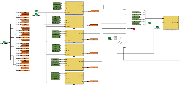
Simulink model

The complete Simulink model is divided into four subsystems: motor, pump, hydraulic fluid dynamics, and one describing pressure.

Results and confirmation

DC machine

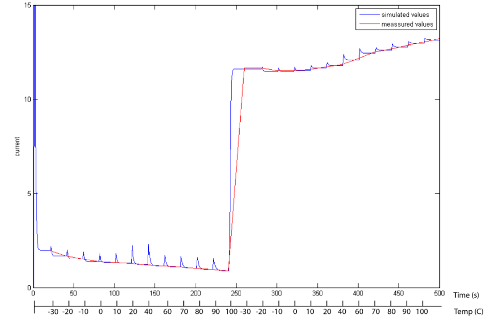
The MATLAB/SIMULINK model is checked against data provided by the manufacturer. Since no dynamic data is available, the model is only tested for static behavior with a constant supply voltage in volts. In the first samples, the engine runs without an external load with a temperature rise of -3 to C. Then the engine is loaded with a constant torque of 20 Ncm, and then the temperature drops again to -30 degrees.

Armature current, in a DC machine, initially without load from -30 to 100 degrees. After 245 samples, a load was applied and the temperature was lowered from 100 to -30 degrees:

The speed of rotation of the DC machine shaft under load and without load from -30 to 100 degrees:

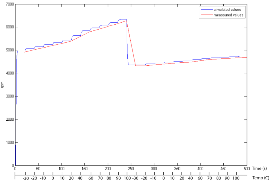
The simulations show good agreement with the figures provided by the engine manufacturer. However, it should be noted that these figures provided by the manufacturer have a discrepancy of 8%. Changing the engine constants will obviously affect the model's performance.

Hydraulic pump

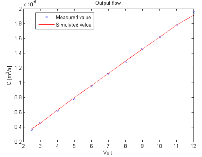
The Haldex company conducted experimental measurements of the useful flow rate of the pump. Although these measurements are purely static, they still confirm the correctness of the simulated static flows.

Measured and simulated static flows from the hydraulic pump:

Hydraulic fluid

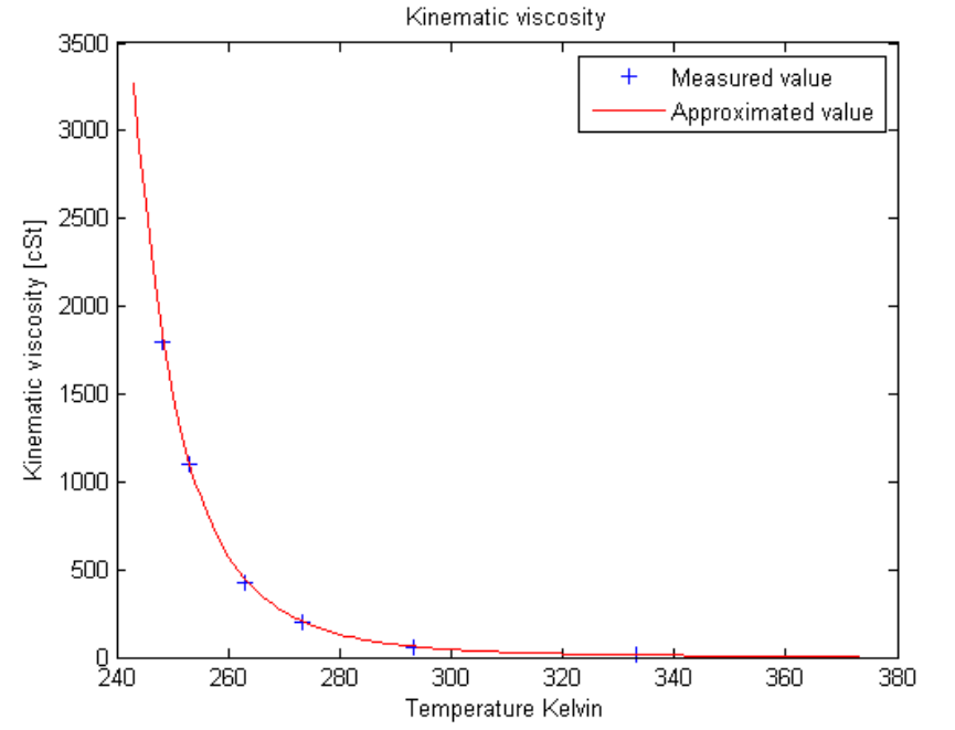
Kinematic viscosity is approximated by a logarithmic function based on measurements made by Haldex. However, since the measurements were available and the density is used to calculate the dynamic viscosity, the function is vital. The volume modulus function is implemented in MATLAB/Simulink, but is not actually used in the current model. This is mainly due to two things. When the elasticity index was introduced in LSC, oil compressibility was already included in the measurement. Another reason is that the hydraulic system is considered completely air-free. Therefore, the hydraulic fluid can be considered incompressible, and compared to the mechanical stiffness in the LSC, this would have an effect on the result. However, the authors of this thesis did not intentionally remove these blocks from the model. If circumstances change in the future, they may be useful.

Kinematic viscosity as a function of temperature:

Density as a function of temperature:

Bulk modulus as a function of temperature and pressure:

Completed model

Measurements were made using a test bench with the actual system. From this setup, the applied voltage, the resulting armature current, and the pressure are recorded. Oil temperature and time are also recorded. This data is then used to compare with the model. Below are step-by-step answers and changes. Finally, one session where the applied voltage is closer to the operating situation is compared with the simulation.

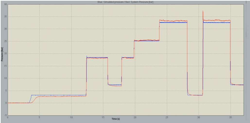
Steps

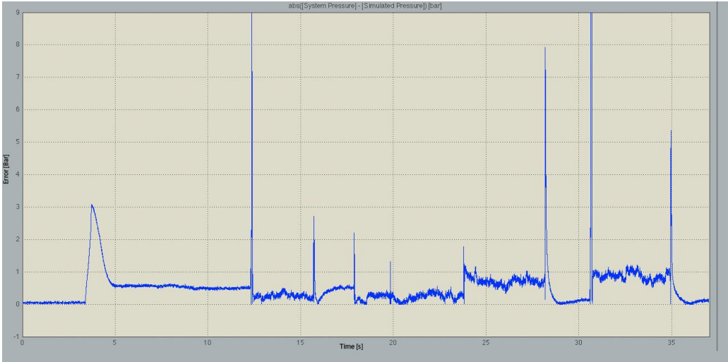
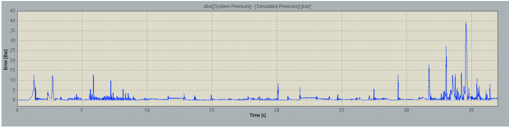
A number of steps are performed throughout the working interval. The following figures measure the error between the actual pressure and the simulated one.

Measured pressure (red) and simulated pressure (blue):

Pressure error:

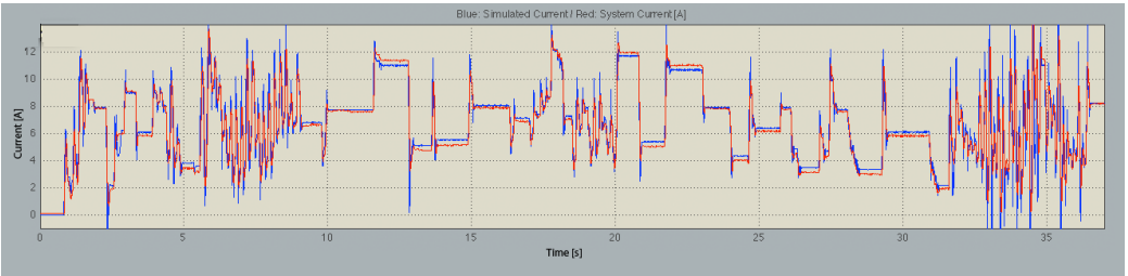
Measured current (red) and simulated current (blue):

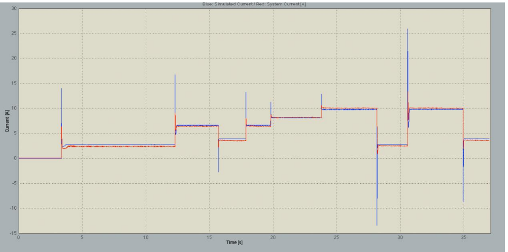
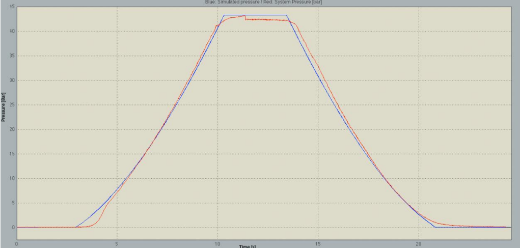
These comparisons show that the pressure build-up in the simulation is somewhat rapid. However, once higher pressures are reached, above 5-7 bar, the simulation closely matches the actual data. The current exhibits the same characteristics; at lower torque and pressure the armature current is not quite accurate, but more accurate at higher pressure.

Ramp

As the armature voltage is slowly increased and then decreased, the system and model show the following characteristics depicted in the following figures.

Measured pressure (red), simulated pressure (blue):

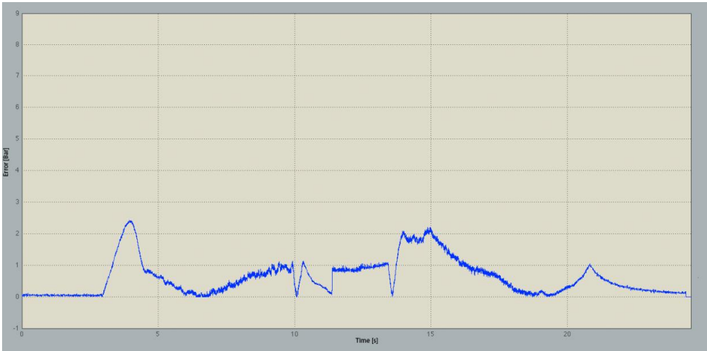
Error between actual and simulated pressure:

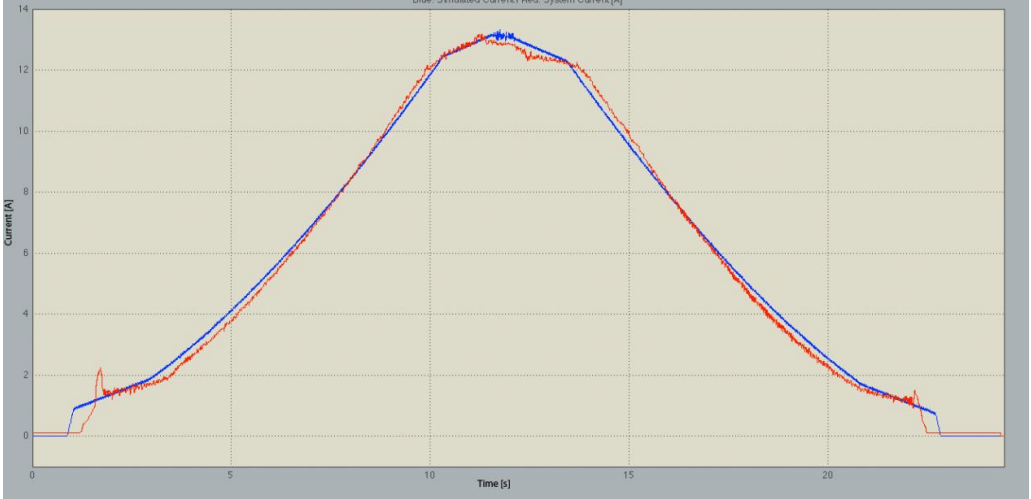
Simulated current (blue) and measured (red):

Pressure increase, when the pressure starts to rise:

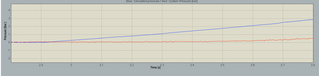
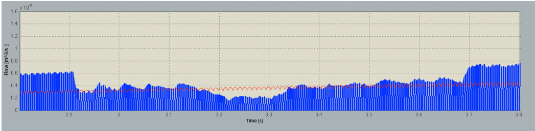
The flow from the pump (red) and the flow coming out of the hole on the arms of the lever (blue):

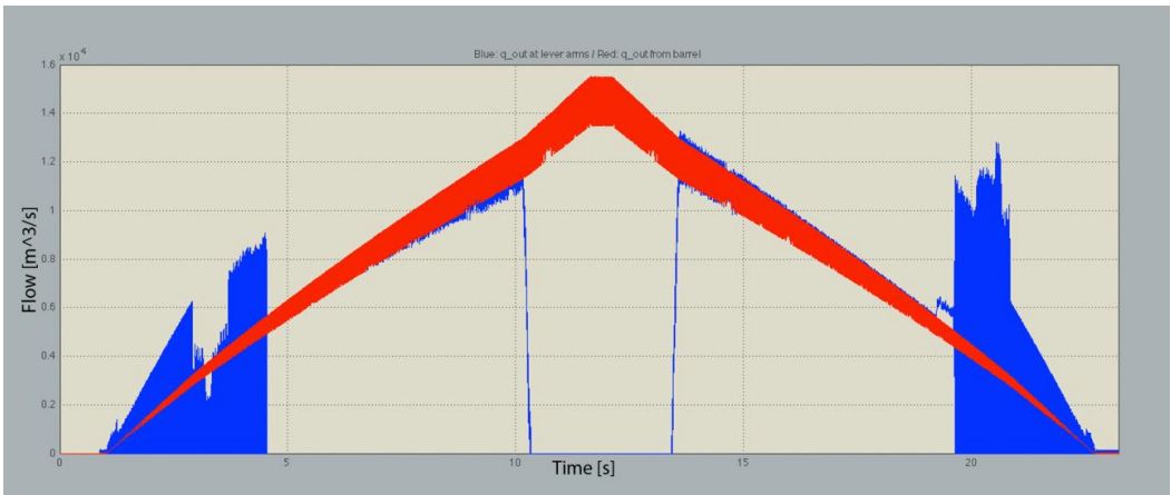
The flow from the pump (red) and the flow exiting through the holes on the arm arms (blue) during a complete cycle of the ramp:

Operational situation

To get an idea of how well the model fits the real operational situation, a third run was performed on the platform. The goal was to simulate a situation when a car skids on ice or snow. This situation was recorded by randomly changing the voltage applied to the motor, alternating high and low frequencies. The pressure error and current comparisons are also presented below.

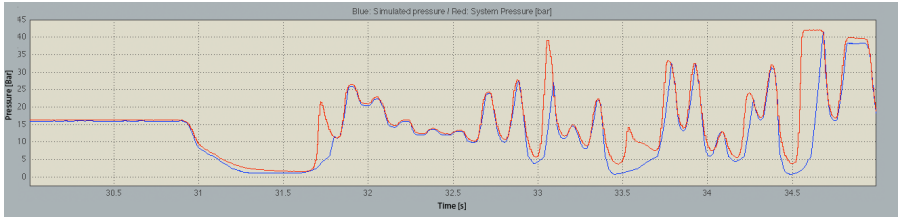
Pressure measurement. Measured pressure (red) and simulated pressure (blue):

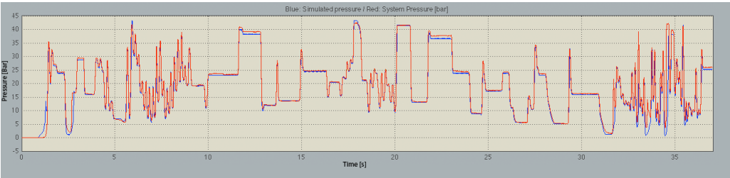
Error between measured and actual pressure:

Current during operation. Measured (red) and simulated (blue):

Not surprisingly, this simulation exhibits the same characteristics as the previous simulations. At low pressure, especially during start-up, the simulation runs faster than the actual system. This section will address the accuracy of the model and examine and compare the input/output data of the full model. Possible areas causing errors will also be discussed.

Accuracy of the model

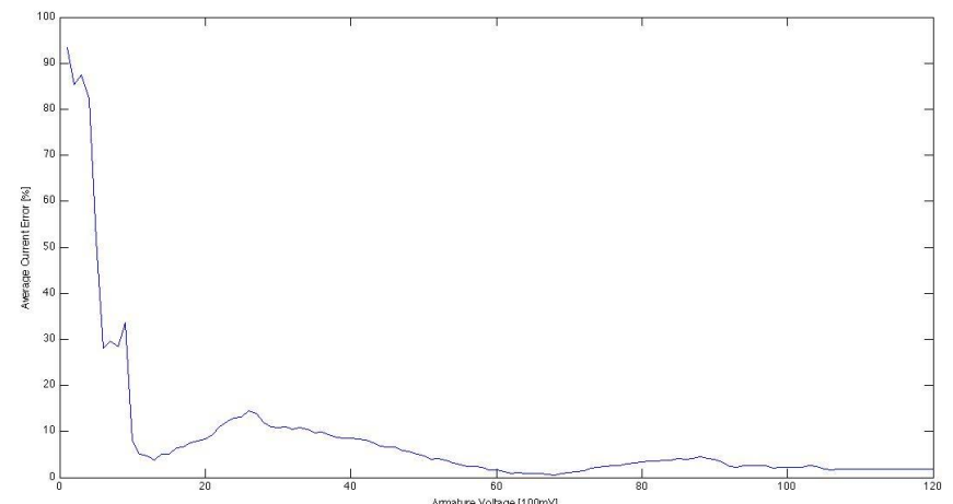
To determine the accuracy of the model, the above two simulations were studied in more detail: the ramp and the operational situation. The percent errors between measured and simulated current and pressure were recorded. The data from these simulations were sorted with respect to the armature voltage, and the average error in the operating region was calculated.

Current ramp simulation error:

Pressure error in ramp simulation:

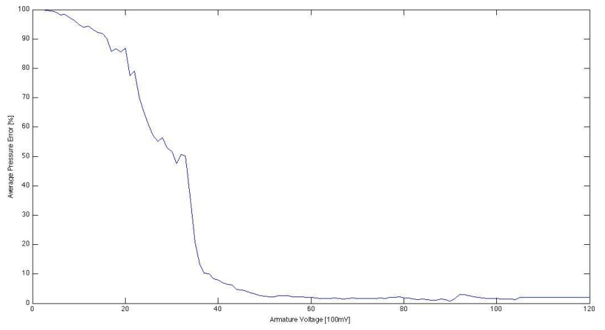
The numbers above are taken from the ramp test cycle. As can be seen in these figures, the error is larger, in fact very large, at lower voltages. This is consistent with previous results, but may be misleading. The absolute error is very small at lower pressures, about 0.05 bar. A more thorough relative error analysis is also performed.

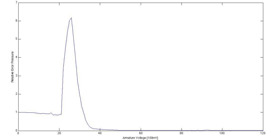
Relative pressure error when modeling the ramp:

The relative error of the current when simulating the ramp:

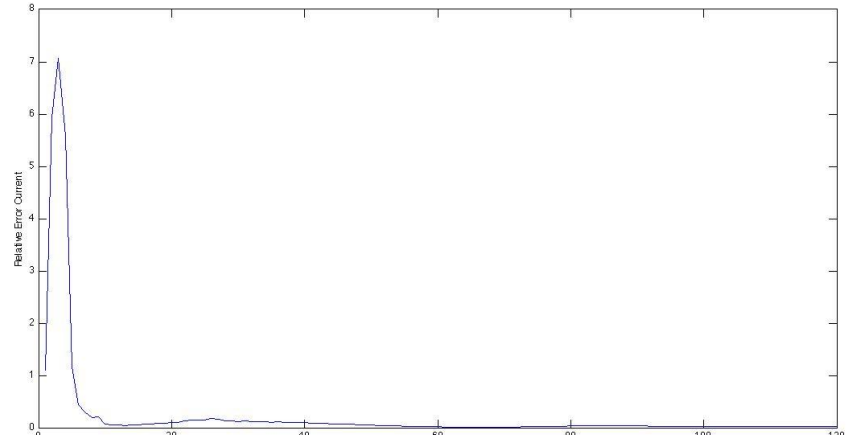
The operative situation shows a similar situation as a ramp. At lower voltages, the percentage of errors is greater, as at higher voltages. In the middle region the error is much smaller, the next section will discuss why.

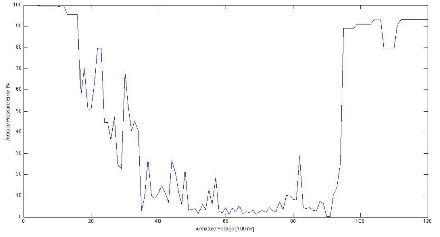
Percentage of pressure error during the working situation:

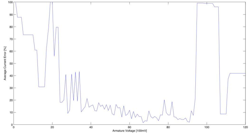
Current error in percentage during the working situation:

Possible reasons for the error

The main reason for the large percentage errors at higher duty cycle voltages is that the voltage rarely reaches these high values during the simulation, and then only in the high frequency regions. This penalizes a model that runs a little slow or a little fast, creating large errors. In addition to current, large transients occur during simulation when voltage changes occur. These transients most likely also occur in a real engine, but due to the relatively low sample rate, they will not be recorded. Below are some more detailed analyzes of operational situation simulation results.

A close-up of the pressure between 30 and 35 seconds:

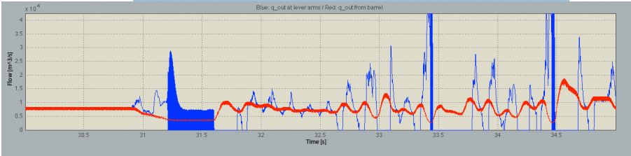
A zoomed-in view of the flows from the pump and levers during the 30-35 second simulation period:

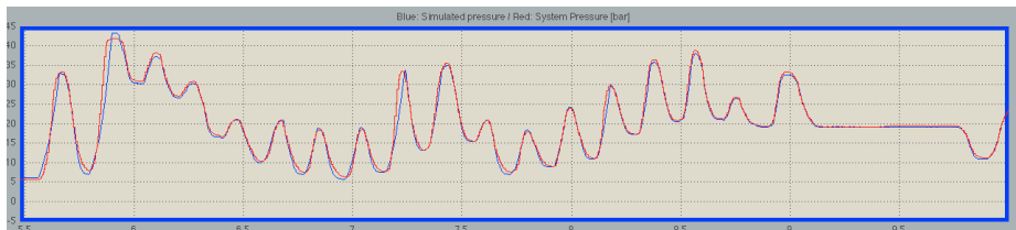
Increased time interval where the simulated result is good. Time [s] is displayed on the horizontal axis, pressure on the vertical axis:

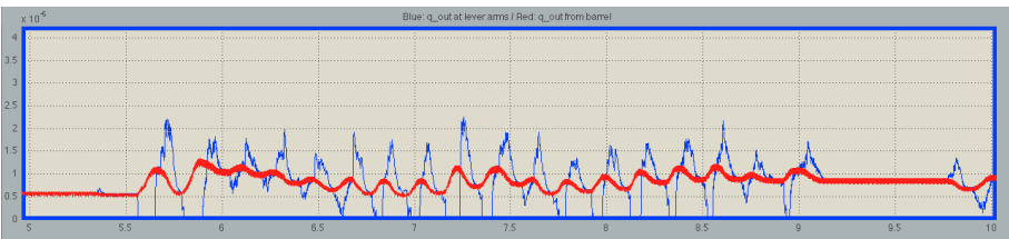
A zoomed-in view of the streams at the same interval as above. On the horizontal axis is the delayed time [s], on the vertical axis is the flow [m3/s]:

This behavior of the flow equation can be a source of error, but the elasticity function can also contribute to errors. Since the function is based on static measurements, changes in the volume of the compartment adjacent to the clutch caused by moving parts are not taken into account. If the volume changes, so does the behavior of the function, which may explain the errors seen at the beginning of the change function.

Conclusion

Simulations on a DC machine show good agreement with values provided by the motor manufacturer, Buhler. Considering that these motor constants have a significant variance, it can be concluded that tuning these values in the model can achieve an even better result. The simulated pump flows are largely consistent with the measurements made by Haldex. The temperature-dependent functions of oil viscosity and density compare well with liquid measurements. A volume module feature was created, but was later abandoned as it was not needed in the current model. However, this function was retained in the Simulink implementation in case the elasticity function was further developed. Comparisons of the full Gen V model with test configuration measurements also show good results. Step response, voltage change, and random voltage measurements all indicate the same result. When higher pressures are reached, the model follows these measurements very closely. When the model generates pressure from zero or very low pressure, it differs from the tests. It has been suggested that this too rapid rise in pressure is due either to uncertain regions in the quadratic equation that governs the pump arms, or to errors in the elasticity function, or to both.

How to check the oil level in the Haldex clutch - read here .

Simulink model

1. Completed model . The model block contains four subsystems; a DC motor block, a hydraulic fluid dynamics calculation block, a pump block and a clutch volume block.

2. DC motor . The block calculates the motor equation described in section 8. The inputs to the block are the voltage u_a and the load torque T_load. The switch routines output zero as long as the shaft speed is zero. This is to prevent the motor from spinning backwards at zero voltage.

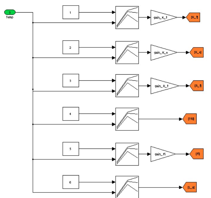
3. DC motor parameters . Engine parameters are contained in lookup tables. These tables are located in the DC_motor block and have temp as input. These parameters make the engine temperature dependent. The coefficients k_t, K_e, R_t and Fi exist to convert from the given units to SI units

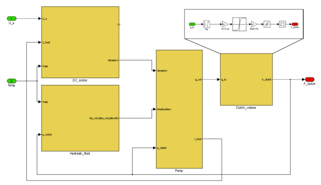
4. Clutch volume . The block contains an integrator representing the volume. It is saturated to prevent reaching negative values. The lookup table contains the coupling elasticity. Output is the pressure acting on the clutch.

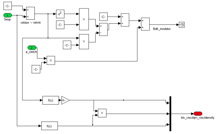
5. Hydraulic fluid . This block calculates the kinematic and dynamic viscosity, as well as the density of the hydraulic fluid. Since they depend on temperature and pressure, P_clutch and Temp are inputs. Bulk_module is also calculated, although the model no longer needs it at this point, so this signal is deprecated.

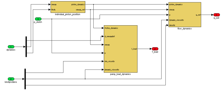
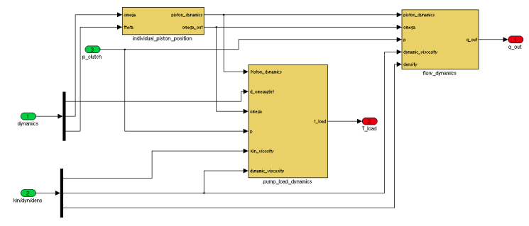
6. Pump . The pump is divided into three subsystems. The individual_piston_position block determines the position, velocity, and acceleration for each piston, sending them to an array called piston_dynamics. The pump_load_dynamics block calculates the load on the motor shaft. Finally, the flow_dynamics block represents the flow entering or leaving the volume adjacent to the coupling piston.

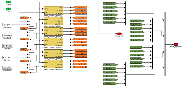
7. Individual piston position . This unit calculates the position, velocity and acceleration for each of the six pistons.

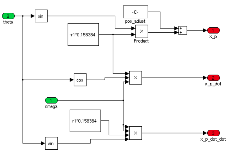
8. Piston dynamics . In this subsystem, piston position, velocity and acceleration are calculated. The pos_adjust constant exists to balance the position equation so that the result is always positive.

9. Piston load dynamics . This block calculates the piston forces for each piston. These forces are then used to calculate the load moment acting on the motor shaft. This is partially calculated in the same force calculation blocks, but bearing losses and friction losses are calculated separately. This is explained by the fact that losses in the bearing depend on the sum of all piston forces.

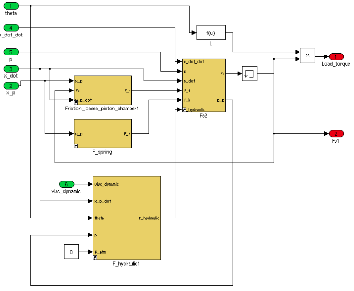
10. Fs (Effort on the skew plate). This block calculates the force F_s, the force from the piston acting on the swashplate. The block also calculates the load torque that this force results in. F_s also determines bearing losses and is thus sent from the block for use in further calculations. The load torque is the sum of the spring force, friction losses, and hydraulic losses multiplied by the lever L. Subsystem Fs2 sums these losses and forces. The L function calculates the leverage.

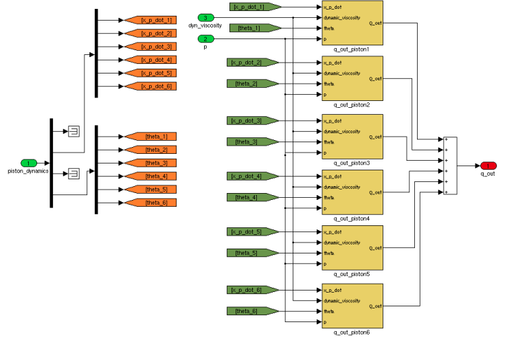
11. Flow dynamics . The block describes the sum of the flows entering and leaving the clutch chamber. A positive q_out can be interpreted as the volume closest to the clutch piston. A negative value can be interpreted as if the flow from the pistons, as well as the volume of the clutch chamber, exits through the hole of the lever.

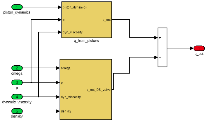
12. Flow from the trunk and leakage flow . The positive flow, i.e. the flow coming out of each piston chamber, is added together to form the total of all these flows.

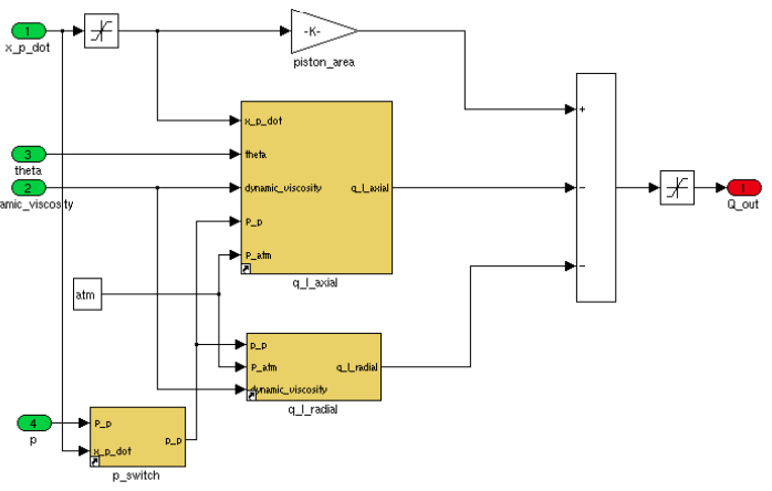
13. Flow from one piston . This block describes the output flow from a single piston chamber through the high pressure side. The flow equation takes the area of the piston, multiplies it by the positive speed of the piston, which creates the flow. This is subtracted from the leakage flows. The p_switch block simply switches the pressure in the chamber according to where the piston is located, on the high or low pressure side.

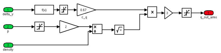
14. Flow from pressure valves/lever . These blocks together calculate the flow through the holes on the levers.

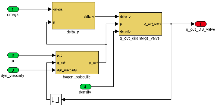
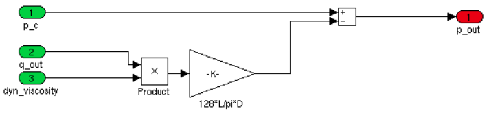
14. Hagen-Poiseuille pressure loss . The Hagen-Poiseuille equation describing channel losses is shown above. The input signal is the pressure in the coupling volume. The output signal is the pressure acting on the ball connected to the lever.

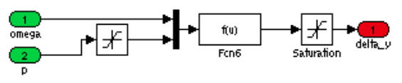
15. Delta U. This function block defines the height of the lever. The inlet pressure is saturated, preventing it from becoming negative. This is due to the fact that the previously described Hagen-Poiseuille loss unit, if the volumetric clutch pressure is zero, will force the pressure to reach negative values, which is unrealistic.

16. It flows from the exhaust valves . This is the equation describing the flow through an orifice. The function block at the top of the model calculates the area of this hole. The flux is multiplied by three, since that is the number of holes, and the result is the total flux.